Week 03 — Imitation Learning
← Control and MDPs · Week 3 of 11 · Next: Reinforcement Learning I →
Outcomes
- Explain why supervised accuracy is insufficient for closed-loop imitation.
- Compare behavior cloning, DAgger, and expressive multimodal policies.
- Diagnose distribution shift, mode averaging, and causal confusion.
Prerequisites: notation
Notation for imitation learning (and intelligent/learning systems in general):
| Symbol | Meaning |
|---|---|
| $a_t$ | Action at time $t$ |
| $o_t$ | Observation at time $t$ |
| $s_t$ | State at time $t$ |
| $\tau$ | Trajectory: $\tau = (s_1, a_1, s_2, a_2, \ldots, s_T)$ |
| $r(s, a)$ | Reward |
Example: for a self-driving car, $o_t$ is the camera image, $s_t$ is the car’s pose and velocity, $a_t$ is the steering/throttle command, and $\tau$ is one full drive.
What is imitation learning?
Given a set of trajectories collected by an expert, called demonstrations:
\[\mathcal{D} = \{ (s_1, a_1, \ldots, s_T) \}\]the goal is to learn a policy $\pi$ that imitates the expert’s behaviour.
Behaviour cloning
The simplest approach — treat imitation as supervised learning. Given $\mathcal{D} = \{(s_1, a_1, \ldots, s_T)\}$, for a deterministic policy, regress onto the expert’s actions:
\[\min_\theta \; \frac{1}{|\mathcal{D}|} \sum_{(s, a) \in \mathcal{D}} \lVert a - \hat{a} \rVert^2, \qquad \hat{a} = \pi_\theta(s)\]then deploy $\pi_\theta$ on the robot.
Does it work?
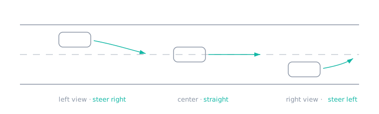
Sometimes, yes — see End to End Learning for Self-Driving Cars (Bojarski et al., 2016), which trained a CNN to map raw camera pixels directly to steering commands.
Trick: “data augmentation”
Bojarski et al. add fake data that illustrates corrections, using side-facing cameras: the left/right camera views look like the car has drifted off-centre, so they are relabelled with the corrective steering command.
The upper bound of behaviour cloning
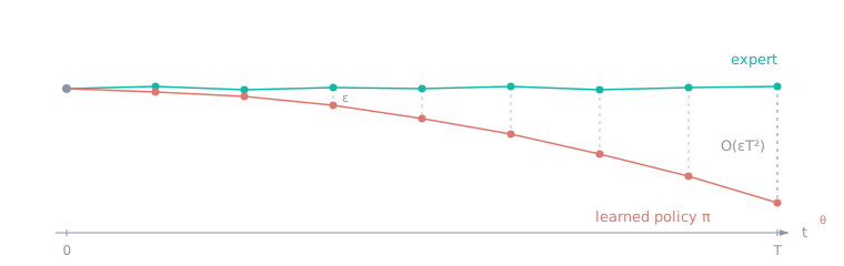
The policy makes a small mistake ($\epsilon$ per step), lands in a state the expert never demonstrated, and makes a bigger mistake there. Over a time horizon $T$, this distribution shift causes the error to compound quadratically:
\[\mathbb{E}[\text{cost}] \in O(\epsilon T^2)\]See A Reduction of Imitation Learning and Structured Prediction to No-Regret Online Learning (Ross et al., 2011).
Addressing compounding error: DAgger
How can we make $p_{\text{expert}}(s) = p_{\pi}(s)$ — i.e. states visited by the expert $=$ states visited by the policy?
Idea: instead of being clever about the policy, be clever about the data — make the dataset cover the states the policy actually visits.
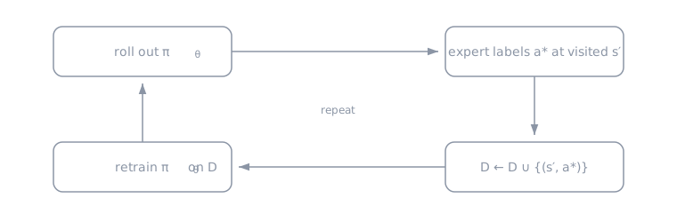
- Roll out $\pi_\theta$ on the robot.
- Query the expert: label the visited states $s^{\prime}$ with expert actions $a^*$.
- Aggregate the corrections with the existing data: $\mathcal{D} \leftarrow \mathcal{D} \cup \{(s^{\prime}, a^*)\}$.
- Update the policy: $\theta \leftarrow \arg\min_\theta L(\pi_\theta, \mathcal{D})$, and repeat.
The good
- Lets the human take control — the true expert.
- Paradox: it works better if the data contains more mistakes and recoveries.
- Hence the algorithm converges: $p_\pi(s) = p_{\text{expert}}(s)$.
- Achieves $O(\epsilon T)$ error instead of behaviour cloning’s $O(\epsilon T^2)$.
The bad
- How do we detect when an intervention is needed?
- Hindsight labelling and expert queries are difficult — this is not ideal in practice.
Example: Waymo self-driving safety drivers (teleoperators) take over when needed, and those interventions become labelled recovery data.
Why might we still fail to mimic the expert?
- The policy’s action depends only on the current observation, but human behaviour may be affected by past observations, emotions, privileged information, etc. (non-Markovian behaviour).
- Human observations $\neq$ robot camera observations — the expert may see and sense things the robot cannot.
- The expert’s action distribution is multimodal, and an MSE policy averages the modes — see below.
Why the MSE policy fails: mode averaging
Demonstrations are multimodal: faced with a tree, half the experts swerve left and half swerve right, so the true action distribution $p(a \mid s)$ has several modes. Minimizing MSE is maximum likelihood under a single Gaussian, so the optimal prediction is the conditional mean:
\[\pi_\theta(s) = \mathbb{E}[a \mid s]\]and the mean of “left” and “right” is “straight into the tree” — an action no expert ever took.
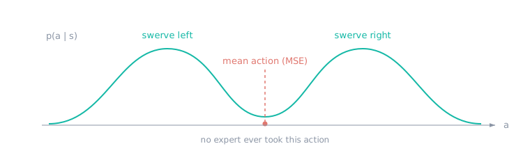
Concretely, if the expert’s actions follow a mixture of Gaussians,
\[p(a \mid s) = \sum_{i=1}^{k} w_i(s)\, \mathcal{N}\big(a;\ \mu_i(s), \Sigma_i(s)\big),\]the MSE-optimal policy outputs $\sum_i w_i \mu_i$ — which can land in a near-zero-probability valley between the modes.
Expressive policies
Fix: replace the implicit unimodal Gaussian with a distribution class that can represent multiple modes.
- Diffusion policies: start from Gaussian noise and iteratively denoise it into an action, conditioning every step on $s$. Extremely expressive; the cost is inference-time compute — many denoising steps per action. (Diffusion Policy, Chi et al., 2023)
- Autoregressive discretization: discretize each action dimension into bins and predict one dimension at a time with a softmax — a language model over action tokens: $\pi_\theta(a \mid s) = \prod_d \pi_\theta(a_d \mid s, a_{1:d-1})$. A categorical can put mass on any bins (arbitrarily multimodal), and autoregression keeps the bin count linear in the action dimension instead of exponential. Costs resolution to the binning. (e.g. RT-1)
- Latent variable models (CVAE): feed noise through the network, $a = \pi_\theta(s, z)$ with $z \sim \mathcal{N}(0, I)$ — different samples of $z$ select different modes; trained with a variational lower bound. (e.g. ACT)
- Mixture of Gaussians (MDN): the network outputs $k$ weights, means, and covariances: $\pi_\theta(a \mid s) = \sum_{i=1}^{k} w_i(s)\, \mathcal{N}\big(a; \mu_i(s), \Sigma_i(s)\big)$. Simple and expressive, but you must predefine the number of modes $k$.
Scaling control to “any” task
How do we go from one policy per task to one policy for any task?
- Single task: $\pi_\theta(a \mid s)$ — one policy per task, nothing shared.
- Task-conditioned: $\pi_\theta(a \mid s, z_{\text{task}})$ — condition on a task ID (one-hot, or a language embedding). One network, data shared across tasks — but only for a predefined list of tasks.
- Goal-conditioned: $\pi_\theta(a \mid s, g)$ — condition on a goal state $g$ (e.g. an image of the desired outcome). “Any task” becomes “reach any goal state”. Bonus: hindsight relabelling — whatever state a trajectory actually ended in is a valid goal for that trajectory, so every trajectory supervises goal-reaching for free.
Caveat: goal-conditioning only covers tasks expressible as reaching a state — “wave hello” or “keep the cup upright while moving” don’t map cleanly to a single goal state.
Dataset and architecture decisions
- Store observation timestamps, action timestamps, control frequency, and episode boundaries.
- Split by trajectory or scene—not individual frames—to avoid leakage.
- Normalize actions with training-set statistics and record the inverse transform.
- Choose whether the policy sees a frame, stacked frames, or recurrent history.
- For visual policies, compare frozen pretrained features with end-to-end training.
Failure modes
- Validation loss falls while closed-loop success collapses.
- Mean regression averages two valid modes into an invalid motion.
- The policy keys on gripper state, background, or demonstrator artifacts.
- Demonstrations show success paths but no recovery behavior.
Paper discussion
Contrast the diagnosis in Causal Confusion in Imitation Learning with the empirical case for pretrained visual representations in Pari et al..
Build milestone
Collect or synthesize demonstrations, train behavior cloning, then introduce initial-state noise. Add either DAgger or recovery data and compare closed-loop success—not just validation loss—over three seeds.
Plot performance against perturbation magnitude and dataset size. Include the expert, a random policy, and behavior cloning before claiming the interactive method helps.